
Variability and Randomness within Classroom Activities
A classroom activity with randomness in it is always a little dangerous. It’s also essential. Students need to see that math doesn’t always give the same answer. And students also need to see that with randomness, the results are often stranger than we expect.
Suppose you’re demonstrating that the probability of rolling each number is 1/6 when you roll a die. You have each student roll the die 36 times and record the results, predicting that on average, each number will come up 6 times. What will happen? These five graphs show actual results from this process.
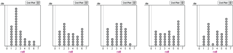
The second and fourth graphs are sort of even, but the other three look decidedly wrong. The problem is that we poor humans expect things to “even out” faster than they do. This expectation is the source of the “gambler’s fallacy”: if you had just rolled the middle graph, you might think that the die was loaded, so that in the next 36 rolls, you'd continue to get fewer sixes. Or you may think that six is “due,” so you expect results more like the graph on the far right.
But dice have no memory: the probability of rolling a six is still 1/6, no matter what. How does that relentless constancy fit with those hinky graphs?
The answer is in the “Law of Large Numbers.” If you kept rolling, you would get closer and closer to the expected, even distribution. Here we see graphs of 36, 72, 100, 1200, and 6000 die rolls:
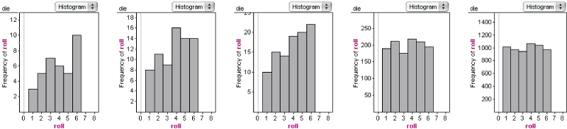
Looking at the first five graphs (copied from above), we see that “variability” goes beyond the idea that a die gives different results when you roll it. Even the pattern of the results—the distribution of die rolls—changes in unexpected ways. This variability carries over into data that are not simple die rolls. Here is a dot plot of the heights in centimeters of 36 12-year-olds.
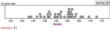
What would we say about the distribution? For one thing, we’d say there was a big clump between about 160 and 163 cm. But is that a “real” feature of the distribution? Here is a different sample of 36 from the same population.
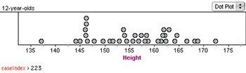
Now the most salient feature is that spike near 146. But the distribution is not completely different: the individual values have changed, and show a different pattern. But the mean and median are pretty much the same between the samples, and the overall spread is about the same.
By the end of high school, we want students to develop intuition about what kinds of features look real (that is, what features will remain when you re-roll or take a different sample) and which are probably the result of random fluctuation. At this stage, we are helping students develop that intuition by showing them examples—examples that arise naturally when you contrast different groups’ results.
Streaks in Coins
Here is a famous example you’ll see if you hang around data long enough.
Suppose Aloysius flips a coin 100 times, recording the heads or tails each time. You’ll have 100 letters in a row, H or T.
Now suppose Penelope makes up 100 coin flips, writing down H or T in a manner she thinks is random, like a fair coin.
You, the teacher, can learn to distinguish real data from fake with astounding accuracy. How?
Humans, trying to be random, avoid streaks. We think that having, say, HHTTTTTTTTHH, in the sequence, is unrealistic. So we alternate more.
In fact, 80% of the time, there will be a streak of 6 or more in a sequence of 100 coins. And 30% of the time, you’ll see a streak of 8 or more.
Here is an internet page that has more information on streaks of heads or tails, and a simulation:
http://demonstrations.wolfram.com/ConsecutiveHeadsOrTails/