
Probability Basics for Middle-School Teachers
The standards for probability at grade seven deal with theoretical and empirical probability, probability models, and compound events.
Much of this material is common sense or things you already know. You may need a refresher on the vocabulary, however, and instruction on some of the visualizations that will help you and your students understand what’s going on.
This document will also fill you in on some of the issues in probability and probability theory that come later.
The Quick Summary
Don’t want to read the whole thing? Here you go:
Theoretical probability is when you know what to expect because it has to be that way, like the probability of getting heads when you flip a coin is P( heads ) = 0.5. Empirical probability is from experience: if you toss a paper cup and it lands on its end three times out of twenty, then P( end ) = 0.15.
If you put two or more events together, you get a compound event. Here is the classic question with a classic wrong answer:
If you toss two coins, a nickel and a penny, what is the probability that you get one heads and one tails?
Wrong solution: There are three possibilities: 0, 1, or 2 heads. So the chance of getting one “heads” is 1/3.
You could show that this response is wrong empirically by tossing two coins enough times, or theoretically by analyzing the situation. You can visualize this compound event with tables and tree diagrams.
Here they are:


In these diagrams, you can see that, in fact, there are four outcomes. Two of them have one tail and one head. So P( one head and one tail ) = 1/2.
If that summary doesn’t tell you all you want to know, read on…
Basics
A probability is a number. It represents the likelihood of something happening. Furthermore, it has to be between zero and one.
An event with a probability of zero is impossible; it will never happen. If the probability is small—close to zero—it’s unlikely. If it’s close to 1/2, it’s (literally in the case of a coin) a toss-up. A high probability—close to one—is very likely, and a probability of 1 represents an event that will certainly happen.
There are two ways to figure out a probability: empirically and theoretically. Let’s start empirically.
Suppose that Denise usually arrives in class first. Usually. Not always. You count for two weeks and she was first into the class seven out of ten times. The next day, will she be first? Probably, but not for certain. We can assign a number to how probable it is: 0.7, that is, 7/10.
That’s an empirical probability. It’s based on experience. You look at what happened in the past, and use that to make predictions about the future. A cool thing about probability is that you don't have to make firm, black-or-white, yes-or-no predictions: your prediction is that there’s a 70% chance that she will be first. The "70%" recognizes that you’re not certain, but it lets you be quantitative about how certain or not certain you are.
Vocabulary note: when you count up how many times something happens, the number you get is called a frequency. (This conflicts with the definition in science, where frequency usually means how many times something happens in some time period.) So in ten days, the observed frequency of Denise being first was 7.
A theoretical probability is when you have a way to know the probability from something other than experience. For example, if you roll a die, the probability that you roll a four is 1/6, or about 17%. That’s because there are six numbers on your die, and each of the numbers is equally likely.
Probability Models
Don’t be frightened by the term probability model. It’s best explained by example.
Suppose you have 28 students in your class. You put every student’s name on a card and shuffle the deck. Whoever’s name is on the top card gets the first question. What’s the chance that Emmitt is first? 1/28.
You have just used a probability model. You have assumed that each card is equally likely because you shuffled. In this case, to generalize, you have used the (common, excellent) model that if you have n things that are equally likely, the probability of each is 1/n.
Not all situations work that way, though. Suppose you put a strawberry and nine blueberries in a bag, reach in, and pull one out. What’s the chance that you pick the strawberry? One-tenth? No way. You can tell the strawberry from the blueberries by feel. Even if you didn’t care, and tried to be fair, they’re different sizes, and that will affect the likelihood of picking the strawberry. So to find the probability, you try it. If you did it 50 times (replacing the fruit each time, of course) and picked the strawberry 17 times out of 50, you would have a 34% empirical probability of picking it. You could use that in a prediction for the future.
This berry experiment also uses a probability model, this time an empirical model based on observed frequencies.
Using and Evaluating Probability Models
Again, let’s use an example.
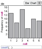
Suppose you have a die that you suspect might be loaded. The probability model for a fair die is that each face has a probability of 1/6. So you take the suspicious die and roll it 60 times. The “expected frequency” for each number is 10. Ten ones, ten twos, and so forth.
But that’s not what you get. Is the die loaded? Not necessarily. After all, even if you rolled a fair die 60 times (there’s no such thing as a fair die, but we can still imagine rolling one…) you probably would not get 10 of each number. So you have to decide if the distribution of results is far enough away from what you “expect” that you have evidence that the die is not fair. (The illustration is from 60 rolls of a fair die.)
At grade seven, you will make this assessment qualitatively—by “feel.” In more advanced statistics, you do the same thing, except that you make that “far enough” criterion quantitative.
Another example: throughout the season, Esme has hit 60% of her free throws. During the latest game, she came to the line 10 times and hit eight. That’s 80%! Did she have a “hot hand,” or is this something we can expect just from randomness? The obvious probability model is that each free throw has a probability of 60%. We might evaluate the model by simulating sets of ten free throws at 60%. The most common results will be 6 “successes,” but how often will we get 8 good free throws out of 10? That’s the question. If "8 out of 10" happens frequently, we can say that Esme's performance is consistent with our model. But if we never see 8 hits out of 10 in 100 tries—100 simulated games of 10 free throws—we’d be reasonably sure that for the latest game, the 60% model didn’t work.
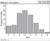
The illustration shows the results of 100 simulated games of 10 free throws each. Eight hits is unusual for Esme, but not super-rare.
Almost Basics
So far we’ve been pretty informal. Let’s take a moment and add some more formal math, using our examples about Denise, who is often first into the classroom, and rolling a die:
- Notation. We often refer to a probability using capital P, and indicate what it’s a probability of in parentheses, as in P( Denise is the first student to enter the classroom ) = 0.7
Learn to read the open parenthesis as “of.” So you say, “P of ‘Denise is first’ is 0.7.” When you understand the context, you can shorten the thing in parentheses:
P( Denise ) = 0.7. - Addition rule. If you know the probabilities of two outcomes, the probability that one of them happens is the sum of their probabilities. So if the probability of rolling a four is 1/6 and the probability of rolling a two is 1/6, the probability of rolling a four or a two is 1/6 + 1/6, or 1/3. And the probability of rolling an even number—two, four, or six—is 1/6 + 1/6 + 1/6, or 1/2. Using our notation,
P( even ) = P( two ) + P( four ) + P( six ).
This is common sense, but there’s a caveat: for this addition rule to work, the outcomes you're looking at can’t possibly occur simultaneously: they must be mutually exclusive. This issue should not come up at Grade 7: as long as you keep it simple—in this case, you can’t roll a two and a four on the same roll with one die—you’re OK. But if you think about cards, and ask, “What’s the chance that the card I draw is a spade or a face card?” You can’t just add 1/4 and 3/13. - Adds to one. If we know the probability that Denise enters the classroom first, we also know the probability that Denise is not first. In this case, it’s 0.3. After all: either she’s first or she isn’t. That’s certain! So:
P( it’s Denise ) + P( it’s not Denise ) = 1,
Therefore the probability that it’s not Denise is 1 – P( Denise ), which is 1.0 – 0.7 = 0.3.
- P(something doesn’t happen) = 1 – P( it happens )
Applying that principle to dice,
- P( rolling something other than a four ) = 1 – 1/6 = 5/6.
If this principle seems painfully obvious, it is. But it’s useful because sometimes it’s easier to figure out the probability of something not happening than the probability that it happens. We’ll see an example later.
Disturbing Background Issues
Probability may seem simple so far, but there are lurking complexities. As teachers, we might downplay some issues for the sake of simplicity. But they’re still there and may come up in the classroom. Here are a few:
- The next day, Denise is first again. Is the empirical probability still 0.7? Nope. Now we have 11 data points, and she’s been first 8 out of 11 times. So the empirical probability has increased from 70% to 8/11, or almost 73%.
- You mean that the chance that she will be first actually changed? Yes and no. Our calculation changed, but you can think of an empirical probability as being an estimate of some unknown true probability. After all, the true chance that she’s first may be some other number like 1/10, and she’s just been lucky. The best we can do is estimate. We will never know the true probability, but by observing longer, we can get a better and better estimate.
- So is this different from the dice, where we know that the true chance is 1/6? Actually, no. In fact, the 1/6 is an estimate as well. There is no such thing as a fair die, and no way that P( four ) is exactly 1/6. But because the die is a cube with six faces and we believe that the manufacturer made a good-faith effort, we assume that the true probability is so close to 1/6 that we’ll never roll enough times to be sure that the true probability is not 1/6. (If you have a student who finishes things too quickly, see if that idea slows them down.)
The Prototypical Compound Event
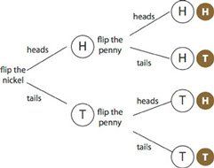
An example of a compound event is flipping two coins: a nickel and a penny. Each one will be heads or tails. The two events are separate; you could think of them as sequential: we’ll flip the nickel and then we’ll flip the penny.
When we flip the nickel, the probability of heads is 1/2. So is the probability of tails. (We’re using the obvious, fair-coin probability model.) It’s the same for the penny, but the result from the nickel has no effect on the penny. The two events are independent. When we follow this through, we see that there are four possible outcomes:
- Nickel heads, penny heads
- Nickel heads, penny tails
- Nickel tails, penny heads
- Nickel tails, penny tails.
These four possibilities are all equally likely—so each one has a probability of 1/4. Is that really true? If it is, we should be able to calculate probabilities we know. For example, we can use our addition rule and calculate the probability of getting heads for the penny alone. The penny shows heads in the first and third possibilities in the list above. So P( penny heads ) = 1/4 + 1/4, or 1/2, which it has to be.
Now suppose we ask, “I’m flipping two coins; what is the probability that I get one heads and one tails?” The right answer is 1/2: it could be either of the two middle possibilities.
The wrong answer is that there are three possibilities: no heads, one head, or two heads. So the probability of one head is 1/3.
What was wrong with the thinking? Because, as plausible as it sounds, we have no reason to believe that zero, one, and two heads are equally likely. We do, however, have reason to believe that heads and tails are equally likely. So, since we know the probabilities of the individual coin flips, we should analyze the compound event (two coin flips) based on those well-understood individual events.
Representing Compound Events
We’ve already used one good representation: a systematic list. A tree diagram is related to that list. We typically make tree diagrams with the tree lying on its side, the “trunk” on the left.
The illustration is pretty elaborate, showing each step along the way. But it doesn’t have to be. The point of the diagram is to help you list all the possibilities; as long as you can do that, the diagram is doing its job.
You could also make a table. If there are two events, you can make one of them into rows and the other into columns:
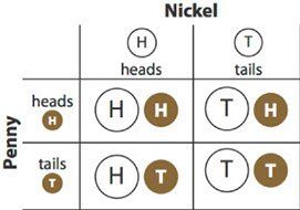
The table organizes the different combinations clearly; you can be sure of listing all four possibilities.
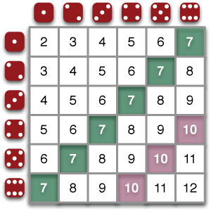
A big advantage of the table is that it makes it easier to list more possibilities. One important application is analyzing the sum of two dice. In this diagram, you can see that there are 36 (equally-likely) possibilities. Six of them give a sum of 7, so the probability of rolling a 7 with two dice is 6/36, or 1/6. The probability of rolling a 10 is 3/36, or 1/12.
Making this as a tree diagram would be a mess. Too many branches!
A disadvantage of the table is that it’s harder (although not impossible) to represent more than two events being combined, whereas in the tree diagram you can just add another layer of branches, for example, if you were flipping three coins.
Area Diagram
Suppose we look at Denise again, who has arrived first in class 70% of the time. What’s the chance that she will be first both of the next two days? This is a compound event: we’re combining two separate events—the two classes on Monday and Tuesday.
We could make a tree diagram or a table, but it’s not clear (yet) how that would help us, because either would look just like the coin visualizations above—but those wouldn’t take the 70% into account. The individual table cells or tree branches would look like they indicate a probability of 1/4. However, the individual outcomes are no longer equally likely, so that 1/4 is probably not correct.
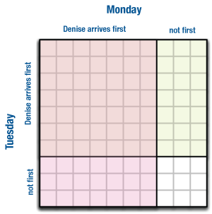
To resolve this problem, make an area diagram, where the distance on each “axis” of the table is proportional to the probability of each event. Students can do this by hand on grid paper.
In the illustration, we’ve used 10 squares, so we could represent the probability nicely. On Monday, 70% of the distance across is for “Denise arrives first.” Likewise for Tuesday and the vertical direction. It’s as if we have ten equally-likely outcomes (ten cards, say) and seven of them are for Denise arriving first.
Now it’s clear: there are 100 possibilities, really, though many of them are the same. And of those, 49 (7 x 7) have Denise arriving first on both days. So the probability is 49/100, or 0.49. (And what’s the chance that she arrives first on only one day? 0.42. Make sure you know how we got that!)
The Multiplication Rule
The example area diagram above suggests a way to calculate the probability without counting little squares: we could multiply the two probabilities in the compound event: 0.7 x 0.7 = 0.49.
This approach also makes sense from a linguistic perspective: 7/10 of the time, Denise arrives first on Monday. Now, what fraction of the time does she also arrive first on Tuesday? That’s 7/10 of that 7/10. And “of”—especially with fractions—suggests multiplication. How do find out what 7/10 of 7/10 is? Multiply them: 49/100.
This powerful generalization works even when you can’t easily draw the diagram on grid paper. Some examples:
- Marco Scutaro batted 0.328 in the 2012 postseason. What’s the chance he gets two hits in his next two trips to the plate? Answer: 0.328 x 0.328, or about 11%.
- The two events don’t have to be the same kind of thing. The chance that Denise is first to class and Scutaro gets a hit in his next at-bat is 0.7 x 0.328, or 0.2296, almost 23%.
- What’s the chance Denise goes a whole week being first? That would be 0.7 x 0.7 x 0.7 x 0.7 x 0.7, which is 0.7 to the fifth power (oooh!), or about 17%.
- We can combine this approach with the “adds to one” rule: What’s the chance that Denise is not first on at least one day in a week? That situation is the same as “she does not arrive first on all five days,” so P( Denise misses at least once ) = 1 – 0.17, or about 83%.
The multiplication rule does not appear in the seventh grade standards, but it’s the direction we’re heading.
When Do You Multiply, and When Do You Add?
Remember: the multiplication rule for probability does not appear in Grade 7. But the moment you get the idea, it’s super-powerful, and you want to use it.
The danger is that you use this rule wrong. A further danger is that you try to memorize some rule about when to multiply and stop thinking about the situation! So some guidance is in order.
You add when you have two possible outcomes for the same event. Think about rolling a four or a two. You add the two 1/6’s to get the probability that this single roll will be four or two.
You multiply when you’re looking at getting specific outcomes in two separate events (making a compound event). If you flip a coin and roll a die, the chance of both getting heads and rolling a four is 1/2 x 1/6, or 1/12. This always works if the two events are independent (one does not affect the other). If they are not independent, multiplication still works but you need to use the correct (conditional) probability.
Here is another revealing way to think about which operation to use: add when you use the word or and multiply when you use and. For example, what’s the chance that I roll four or two on this roll? 1/6 + 1/6 = 1/3. What’s the chance that I roll four this time and I roll two next time? 1/6 x 1/6 = 1/36. Of course, the "or" has to be in the same event, and the two outcomes have to be mutually exclusive. For "and," the two occurrences must be in different events. After all, the probability that you roll a two and a four in one roll of a die is zero.
Connections
This bit of mathematics obviously connects to the statistics students are learning. But it also connects to other content standards:
- understanding number, proportion, and geometry, through its emphasis on numbers less than one—which we represent as fractions, decimals, and percents;
- performing operations with these numbers;
- recognizing probability as a ratio;
- and, if you use the area diagram, areas of rectangles.
- You might get the impression that theoretical probability is better than empirical because it’s more accurate, more abstract, or generally more mathematical—that if you can solve a problem theoretically it’s somehow preferred. That might have been the case once, but with technology we can compute empirical probabilities to any precision we want. And the thinking behind those simulations is just as sophisticated as anything theoretical; it’s just different. The bottom line: you need both.
- About models. We call them models because we hope they’re good representations of reality—that they capture the essential aspects of reality even though they’re not the real thing. So think of them like model trains, say, as opposed to runway models or the latest model of car. A probability model does its best to give you an accurate picture of what will happen—but in real life it often falls short. When we calculate Scutaro’s chance of getting two hits in his next two at-bats, we’re assuming that his batting average is the true probability, and that probability does not change. That’s wrong—but it may be the best we can do.
- Deep mathematical thinkers can sometimes get very philosophical and hair-splitty about things. Revel in it, try to figure out where they’re coming from, see if it’s useful, but don’t let it spook you. A good example: suppose you flip a coin and cover it without looking at the result. What’s the probability that it’s heads? Many probabilists (that’s what they’re called) will say that you can’t answer that—the probability is either zero or one because it has already happened. Others will say that for all practical purposes, the probability is still 1/2.
- Here’s a classic more-advanced probability problem that involves geometry: if you take a piece of raw spaghetti, and randomly break it in two places (making three little pasta sticks), what’s the probability that you can make a triangle with the three pieces?
- Many problems and situations in which you apply probability in real life need a concept called expected value. That’s the average of some numerical result; so the expected value of a roll of one die is 3.5; and the expected value for the number of free throws Esme will make in ten shots at P = 0.6 is six. You analyze gambling games by calculating the expected value of a play of the game; in a casino game, that expected value is always negative. You also use expected value to analyze situations involving risk. So insurance, public policy, health care decisions, and many other fields all involve expected value.